How To Find Missing Values Using Vlookup
After the logical test if the entry is found then a string OK is returned otherwise Missing is returned. Select an empty cell to store the formula and the returned value.
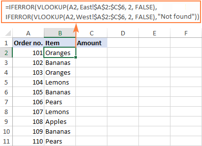
Vlookup Across Multiple Sheets In Excel With Examples
In this example we will check the product names of VL2 with the product names of VL3.

How to find missing values using vlookup. Then the matched values will give us the confirmation using the IF function. In general the VLOOKUP function searches values from left to right in the array table and it requires the lookup value must stay in the left side of target value. Open the VLOOKUP function in the Result workbook and select lookup value.
Missing values from a list can be checked by using the COUNTIF function passed as a logical test to the IF function. 33 rows Using an approximate match searches for the value 1 in column A finds the largest value. We now specify what we need to display in the cell if the row number is not found.
However you can force it to bring the 2 nd 3 rd 4 th or any other occurrence you want. Firstly the lookup value is searched in the particular column of the table array. Now go to the main data workbook and select the table array.
For example if your lookup value is in cell C2 then your range should start with C. Find Missing Values. Find maximum value MAXVLOOKUPA2 Lookup TableA2D10 234 FALSE The formula searches for the value of cell A2 in Lookup table and finds the max value in columns BC and D in the same row.
Remember that the lookup value should always be in the first column in the range for VLOOKUP to work correctly. Under the Functions Library section click the Lookup and Reference drop-down menu and select the. You can check if the values in column A exist in column B using VLOOKUP.
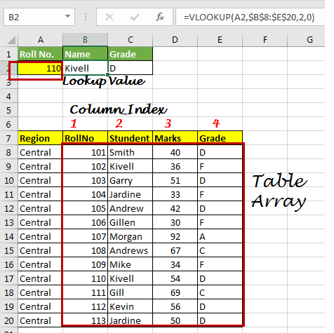
Using VLOOKUP to find duplicate values in two Excel worksheets Make 2 new worksheets titled VL2 and VL3. The Excel VLOOKUP function lookup a value in the first column of the table and return the value in the same row based on index_num positionThe syntax of the VLOOKUP function is as below VLOOKUP lookup_value table_array column_index_num range_lookup. Therefore you need to vlookup backwards in Excel.
Excel Find Missing Rows Between Sheets. We are looking to see if the VLOOKUP returns NA. Select the first blank cell besides Fruit List 2 type Missing in Fruit List 1 as column header next enter the formula IF ISERROR VLOOKUP A2Fruit List 1A2A221FALSEA2 into the second blank cell and drag the Fill Handle to the range as you need.
Press Enter to assign the formula to C2. As you already know Excel VLOOKUP returns the first value it finds in the return column that matches the lookup value. If your companies are in column A on both sheets then you can use a countif or vlookup formula to find the missing companies.
FOLLOW ALONG FILE. The IF function returns the confirmation using the values. Httpsauditexcelcozaproduct-downloadsYouTubeXLVLOOKUP-hands-on-exercises-v2xlsxNext Video- httpsyoutubeXu4Bf3TXIK8 - Previous.
Find minimum value MINVLOOKUPA2 Lookup TableA2D10 234 FALSE. Use a column that is not currently in use and enter this formula on Sheet 1 starting on row 1. COUNTIF A1Sheet 2AA row disappeared in.
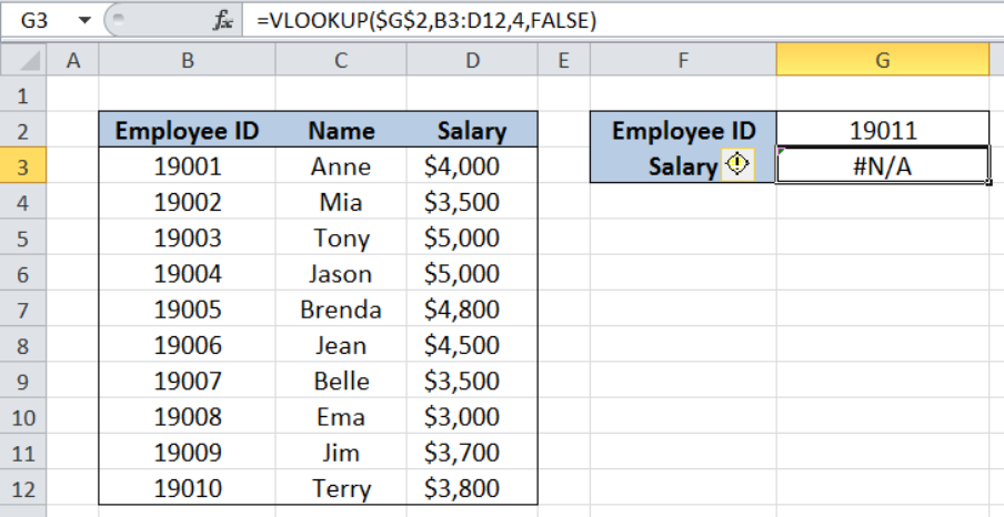
We will construct a formula out of it. Insert the formula in IF ISERROR VLOOKUP A2B2B10011FALSEFALSETRUE the formula bar. You can use Ctrl Tab to switch between all the opened excel workbooks.
In column B of both worksheets create a list of some products name. Next we take the VLOOKUP Function to lookup the ROW number that relates to cell A1 which returns the value 1 in the list of values that are in cells A1 to A20. Summary To compare two lists and pull missing values from one list to the other you can use an array formula based on INDEX and MATCH.
But sometimes you may know the target value and want to find out the lookup value in reverse. If you need to get all duplicate occurrences you will have to use a combination of the INDEX SMALL and ROW functions. Finishing The IF Function.
The formula in D12 copied down is. Select cell C2 by clicking on it. In the example shown the last value in list B is in cell D11.
The range where the lookup value is located. Click the Formulas tab. The column number in the range that contains the return value.
Rexcel - Easiest way to find missing information betweenExcel Details.
![]()
How To Vlookup To Return Blank Or Specific Value Instead Of 0 Or N A In Excel

Doing A Vlookup To Fill In The Missing Columns Produced By Excel S Consolidate Function Excel Learning Consolidation
Excel Vlookup The Ultimate Guide To Mastery


5 Easy Ways To Vlookup And Return Multiple Values

Vlookup Example 5 Lookup Table Computer Technology Excel
![]()
Excel Formula Vlookup If Blank Return Blank Exceljet

How To Troubleshoot Vlookup Errors In Excel
17 Things About Excel Vlookup
![]()
How To Vlookup To Return Blank Or Specific Value Instead Of 0 Or N A In Excel

How To Use Vlookup Vlookup Exact Match Vlookup Approximate Match Exce Tutorial Microsoft Excel Excel
How To Troubleshoot Vlookup Errors In Excel
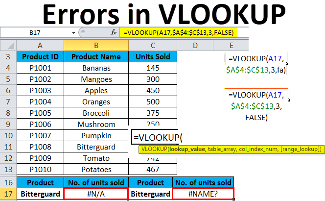
Vlookup Errors Examples How To Fix Errors In Vlookup
Vlookup With Table Array 5 Best Practices Excelchat
How To Use Vlookup With An Excel Spreadsheet Excel Spreadsheets Spreadsheet Excel Formula
Vlookup To Find The Closest Match Last Argument True

Excel Formula Find Missing Values Exceljet
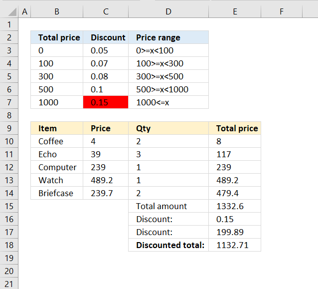
Use Vlookup To Calculate Discounts Commissions Tariffs Charges Shipping Costs Packaging Expenses Or Bonuses

Excel Vlookup Function Vlookup Excel Microsoft Excel Excel Tutorials

How To Vlookup And Return Matching Value In Filtered List